
What is OSPF?
OSPF is a widely used dynamic routing protocol among many companies today. Unlike with static routing, dynamic routing protocols aren’t dependent on human input to calculate and choose the various hops between routers. A network engineer tells the equipment to use OSPF by entering a few commands, and the routers automatically calculate the best paths based on the topology, reducing the need for manual route entry. Information is exchanged between the routers, a map of the entire network is created, and each router makes its own copy of it. The routers then use a calculation called Dijkstra’s algorithm to find the shortest paths between the devices, and the setup is complete. Hello messages are typically sent every 10 seconds from each OSPF-configured interface, and changes are made accordingly. Sometimes, a device goes down, and neighboring devices use a 40-second dead timer. Suppose the device is down for longer than 40 seconds. In that case, new information will be sent throughout the network, signaling a configuration change, and all other devices will update their maps accordingly. If the topology changes, each router creates a new map, performs additional calculations, and continues forwarding network traffic. Let me try to explain the process with an analogy.
One Map Many Islands
Suppose you’re living on an island in an area of islands. Let’s call this area Area 0. Typically, OSPF organizes routers into areas. Many islands are nearby, but we will only focus on the immediate area of islands. There may be only four to five individual islands in this area. OSPF can become quite complex when we delve into backbone areas, area border routers, stub areas, and the various types of LSAs exchanged between them. I may go into these topics in a later blog post, but I don’t want to overcomplicate things. All we need to know is the basic idea of how an LSDB (Link State Database) is formed and updated in a single area. Now, back to the analogy. Let’s say someone is trying to determine the best sailing route between a group of islands in an area. He has no way to see beyond any adjacent islands, nor has he made any contact with them. The neighboring inhabitants of these islands can communicate with him, but only in a minimal manner. If you have ever visited a bank and deposited a check, you have likely seen the air tube suction devices at the drive-through, located next to the ATM. You put your check in a small cylindrical capsule, then in a larger tube, and it is sent to the bank teller.
Suppose a series of tubes like the ones at your local bank connects all the islands and serves as their sole means of communication. On each island, one set of tubes sends information, and the other receives it. People on the individual islands can all write down and transport immediate details about their island and its surroundings to different islands in the area. When this information is exchanged, all of it can be compiled to form a detailed map of the region. These pieces of the map are referred to as LSAs, or link-state advertisements. Let’s assume the people on the islands haven’t sent or received any messages yet. There has been no communication between the islands. During this initial stage, several necessary steps must take place to establish communication between the islands, allowing for the proper exchange of map pieces. Before any contact is made, this state would be referred to as the ‘down’ state in OSPF.
Imagine that to begin communication, a person on one of these islands writes a letter with the word “Hello” on it and sends it out a tube to a neighboring island, hoping for a response. A neighbor receives the ‘hello’ letter. In OSPF, this is referred to as the ‘init’ state. The adjacent island or router has received communication from someone, but they have not yet received a response. Once they receive a ‘hello’ letter back from their neighbor, this is referred to as the ‘2-way’ state. The next stage in the process is called ‘exstart’. In the ‘exstart’ state, the first island and its neighbor determine who will initiate the exchange of the data or map pieces. In the case of OSPF, the routers attempt to build a map of the area; therefore, they send parts of the map as they see it from their perspective of the network. The next state is called the ‘Exchange’ state. This is just like it sounds. The islands begin sending and receiving map pieces. After this, the ‘loading’ state occurs, during which the islands begin requesting any missing pieces of the map that may not have come through. Finally, the ‘full’ state is reached when all the information has been received, and the islands can now begin determining the best sailing routes by referring to their maps.
Sometimes, depending on the type of OSPF setup, a designated and a backup designated router are determined. Imagine a person on one island has been designated to collect all the map information and redistribute it to the other islands. Only one person is chosen to do this. This is to prevent the tubes from becoming clogged with map pieces or LSAs. Let’s call this person DR. DR is responsible for collecting all the combined LSAs from the other islands and transmitting them to the different islands. Each island then compiles the LSAs into identical maps of Area 0 called an LSDB or link-state database. This is what is happening with the stages: down, init, 2-way, exstart, exchange, loading, and full. Sometimes the map needs to be updated because other islands are constructed, canals are carved, or ports are shut, creating more or less efficient routes. When this happens, the people on the islands create new puzzle pieces and pass them off to DR. DR has a partner on a different island named BDR, who is on standby. The BDR is available in case the DR needs to take a break or if communication with them is lost. Perhaps the air tubes to his island are no longer functioning, or they have broken for some reason. The BDR assumes the DR’s role and begins collecting information from the adjacent islands to redistribute throughout the area. The map or LSDB may be different now that DR is out of the picture, and the other devices take note of this. Once the map has been created, the islanders perform complex calculations using Dijkstra’s algorithm again and determine the shortest routes from each island to all the other islands. Dijkstra’s algorithm is quite complex, and it would be too lengthy to explain in this article. I may create a blog dedicated solely to presenting it in the future.
Configurations
In this case, the DR would be R4, but that’s only if I had used a switch to connect the routers to a single subnet and used a /29 prefix or a lower prefix. Because there is no switch between the routers, each pair of interfaces must be configured as /30 subnets, resulting in only two usable host IP addresses. This means that each link will form its own network segment. Therefore, each subnet has its own separate DR and BDR with no DRothers.
What we typically think of as a point-to-point connection in a router setup is still treated as ‘broadcast’ with an Ethernet connection in OSPF. If I had used an older serial connection, the connection type would be displayed as point-to-point, and no DR or BDR would be selected.
With OSPF’s default reference bandwidth of 100 Mbps, any interface with a bandwidth of 100 Mbps or greater is assigned an OSPF cost of 1, unless it is manually adjusted. Configuring a reference bandwidth ensures that 1-gigabit interfaces have a lower cost than 100 Mbps interfaces, rather than all interfaces having the same value of 1. This affects the choices the routers make regarding route selection, as otherwise, there would be no difference in the routes selected. In the running configuration on each interface, I configured OSPF to use 10.0.0.0 with a wildcard mask of 0.0.255.255, or a /16 subnet mask. I chose a /16 prefix because in this simple route, the third octet of each network is where they differ. If I had used a /24 subnet or a higher subnet, I would have had to enter every network address for each interface manually. Doing it this way is less specific, but it ensures that all IP addresses are included in OSPF.
Finally, I included a default route to a mock router labeled ‘internet’. The default route is in place as a backup, in case a packet outside the 10.0.0.0/16 range needs to be forwarded to another destination. The ‘internet‘ or default router intercepts any traffic sent to the least specific configured route on the devices. This route is labeled 0.0.0.0 0.0.0.0 with a hop to 192.168.3.2. For some reason, this default route also did not forward to the other devices using the ‘default information originate‘ command in Packet Tracer, so I had to configure a route from R1 to R2 with the same ‘default information originate‘ command. Once I did that, all the other devices updated their routing tables with the default route. The main takeaway from the lab is evident when you ping from PC1 to PC2 in simulation mode. Notice that the packets always go from R1 to R3 to R4 and back along the same path. This is because the gigabit interfaces on R3 have a cost of 1, as opposed to the Fast Ethernet interfaces on R2, which have a cost of 10. The routers will always choose the cheapest path. That is all I have for this particular lab. I plan to explore this in greater detail in a future post. As of right now, I’ve had about as much of OSPF as I can take. It’s not a very easy protocol to understand. Once you think you have a solid grasp on it, new concepts come up and destroy your perceived understanding of it. I have included a link to my GitHub repository as usual. Please feel free to experiment with it and explore the configurations. Have a great day, and thank you.
GitHub Lab Link: georgebatton/OSPF: OSPF Routing Setup