

I would like to apologize for the complex-looking image accompanying this post. I promise it’s not as complicated as it looks. We are currently discussing static routing, which is the process of manually preconfiguring a route that network traffic will take from one device to another. Let’s use an example to illustrate what’s actually happening. We are currently at home at PC1, and we want to travel to our friend’s house across town at PC2. We have a package to pick up and bring home. Much like your address at home, our home PC has an address on the street 10.0.1.0. This is also referred to as a network address. Maybe my friend lives on Elm Street, but that’s not enough information for me to find his house.
No one, when giving directions, says to their house, ‘I live on Elm Street’ and leaves it at that. They will likely say, ‘I live at 1237 Elm Street’. In our example, we might think, ‘Oh my friend lives at PC2 and I live at PC1. Unfortunately, this is a very vague description and insufficient to know where we’re going. It would be like asking where your friend lives and him telling you that he lives in a red brick house. Okay, there are millions of red brick houses in the country. Which one?
Your computer will ask the same question, but instead of requesting something like 1237 Elm Street, it will ask for 10.0.2.1. The .1 at the end is similar to the 1237 and the 10.0.2. is like the ‘Elm Street’ part of the address, except it says 10.0.2.0.
Now imagine we call our friend to ask for directions to his (or her) house and he answers: “Okay, first: 10.0.2.0/30 [1/0] via 192.168.3.2, and then 10.0.2.0/30 [1/0] via 192.168.2.2.” You would likely have no idea what he was talking about. Unfortunately, this is similar to what network engineers must interpret when examining routing tables, as it’s the exact output we see on the routers along the path from our PC to our friend’s PC.
Now imagine if he rephrased it like this: “At the first stop light, turn right on 192.168.3.0 street. Okay, so if you look at the map coming from PC1, there is a box labeled SW1. That’s a switch, and you don’t have to worry about it. Just go past it and on to the intersection labeled R1 with the stoplight. This intersection is also referred to as 10.0.1.2 and serves as your default gateway or router. So, you’re still on our street 10.0.1.0, but now facing right to get to the next intersection.” He continues, “Go straight until you get to the intersection at 192.168.3.2 (R3) and turn left at 192.168.2.0 street.”
Finally, “After you pass the intersection at 192.168.2.2, go straight past SW2, it will turn into 10.0.2.0, then you go to house .1.” Whew. So, we finally have a map to our destination. We’re not done yet, though. We still have to know how to get back home to PC1. We have to go back the same way we came. Hopefully, that wasn’t more confusing than the output of the routing table. There’s more jargon in the routing table of R1 that we need to explain. We understand the static route labeled with an ‘S’, but what are all these routes labeled ‘L’ and ‘C’? For instance, on R1, there’s a route:
-C 10.0.1.0/30 is directly connected, FastEthernet1/0
What is this exactly? Take a look at the diagram. This output indicates that the interface F1/0 on the router is directly connected to the network or street 10.0.1.0. Next, we will see this:
-L 10.0.1.2/32 is directly connected, FastEthernet1/0
The L stands for local, and it refers to the address (or house) number 2 of the exact device, PC2, on 10.0.1.0 street.
Additionally, there are two other local and connected routes in the table showing up as:
-C 192.168.1.0/30 is directly connected, FastEthernet0/0
-L 192.168.1.1/32 is directly connected, FastEthernet0/0
-C 192.168.3.0/30 is directly connected, FastEthernet0/1
-L 192.168.3.1/32 is directly connected, FastEthernet0/1
Think of the ‘C’ or connected routes as separate roads connected to the intersection R1, but with different street names. We have two possible IP addresses, 192.168.1.0 and 192.168.3.0, from which to travel on from R1. The .1 is similar to the street number address of the router (R1), just as the .2 is the street number address of your PC.
Okay, so onto getting back home. Let’s make this as easy as possible. Each time you specify a new hop from your current location, you must select your end destination street. In this case, we are currently on 10.0.2.0 street. Therefore, we need to reach 10.0.1.0 street and the house at .1 or PC1 on that street. We need to make only two hops or turns. First, we need to travel from street 10.0.2.0 to 192.168.2.0 street and proceed to the intersection at 192.168.2.1. We then need to turn right onto 192.168.3.0 street and then to 192.168.3.1 or R1’s interface F0/1. Finally, to get home, we need to turn left onto 10.0.1.0 street and go straight through SW1 to the PC at 10.0.1.1.
So if we were trying to pick up a package from our friend, it might be something comprised of many large pieces. Therefore, they may need to be broken up into several separate boxes and reassembled once we have them all back home. It’s also possible that we won’t be able to fit all the packages in our car, so we may have to take several trips. Actually, what’s really happening is that PC2 is sending packages, but the route must first be configured for this exchange to take place.
PC1 might be a client requesting information, such as a website or file from PC2, so a package carrier encapsulates and breaks up the data into smaller packets. Different protocols are used to determine how this data is passed across the route. Perhaps the packages are filled with essential parts and must use a protocol like TCP to ensure they arrive with nothing missing. Alternatively, they may be just bits of data in the form of voice or audio, where you can still probably understand it if some of it is missing. For this kind of data, the packets use a protocol called UDP.
Anyway, we’re getting deeper into this topic than I intended. The main point I wanted to express is how we tell the devices to create these routes. Look at the upper right corner of the diagram. You will find a configuration table that explains the exact configuration on each router required to make this static route possible. The only thing missing is the subnet mask. For instance, on R2 we would enter:
ip route 10.0.1.0 255.255.255.252 192.168.3.1
ip route 10.0.2.0 255.255.255.252 192.168.2.2
Essentially, we are instructing the router to identify the network we are attempting to reach, its subnet mask, and then the next hop to achieve this. Since R3 is a junction between the two networks, it needs two static routes. R1 and R4 only need one next hop.
I hope this explanation made sense. This topic can often be difficult to imagine because the process is invisible to the eye. We need to use images of ideas in our everyday life to gain a better understanding of what’s happening. Just remember that before information can be transmitted from PC1 to PC2, we first have to determine a path to and from the destination, or they cannot communicate.
In the next post, I plan to delve into the mechanics of one of the earliest dynamic routing protocols, called RIP, or ‘Router Information Protocol’. As you can probably imagine, when we are dealing with many PC’s and many networks, trying to configure routes manually can be an almost impossible task. Dynamic routing protocols were designed to tackle this issue. I hope you will join me in the next lab to learn about this.
If you want to play around with this particular lab, I have linked it here:
georgebatton/Static-Routing: Lab Showing Static Routes Configured Across a Network