Finding the Shortest Path
Suppose you are located in a particular city and trying to choose the shortest and easiest path to a different city. You want to map out the most efficient route possible to save on gas, time, and money. If we examine the network setup above, we might envision each router as an individual city connected by various roads. When looking at the map, can you tell me the shortest path from R1 to R6? What about the shortest path from R2 to R5? We can’t go in a straight line, bypassing the roads, as doing so would likely lead us into lakes, rivers, ditches, and other obstacles. Roads, like wired networks for data traffic, have been built to provide a medium for our vehicles to travel.
In wired networking, we also assume that data traffic can only move across physical cables. Sometimes, when driving, we don’t always get to choose the route with the literal shortest distance, as it may involve expensive tolls, increased traffic, reduced speed limits, and other various factors. There might be a physically shorter route for driving from Cincinnati to Chicago, but it could also be on slower back roads. The interstate may be a longer distance, but unlike on back roads, you can drive 75 to 80 miles per hour instead of 25 miles per hour. How do we consider all these factors and select the most efficient routes between cities? To solve this problem, we need a foolproof formula that can calculate the most efficient paths every time. For this, we need Dijkstra’s Algorithm.
Dijkstra’s Algorithm is a mathematical formula discovered by Dutch computer scientist Edsger W. Dijkstra in 1956. Dijkstra was trying to find the fastest path between two points on a graph, and later used an example of finding the shortest distance from Rotterdam to Groningen as an analogy to explain the system. The formula is a systematic method of tracing the possible paths and using weighted edges while keeping track of unvisited and visited nodes. A table of tentative distances is used to keep track of the cost as you add up the distances to the unvisited nodes along the path.
A “tentative distance” is the current best-known distance from the starting router to another router, which may be updated as shorter paths are discovered. You keep track of the visited nodes in the same table and add your previous numbers to any unvisited nodes until you reach your destination. You then trace the route backwards on the table, and you can find the shortest distance on the graph, provided it originates from a visited node. In the image above, you can see the path from R1 to R6 that OSPF calculated using this algorithm. To create an LSDB that maps the system, OSPF utilizes Dijkstra’s Algorithm to determine the shortest path between routers
Understanding the Algorithm
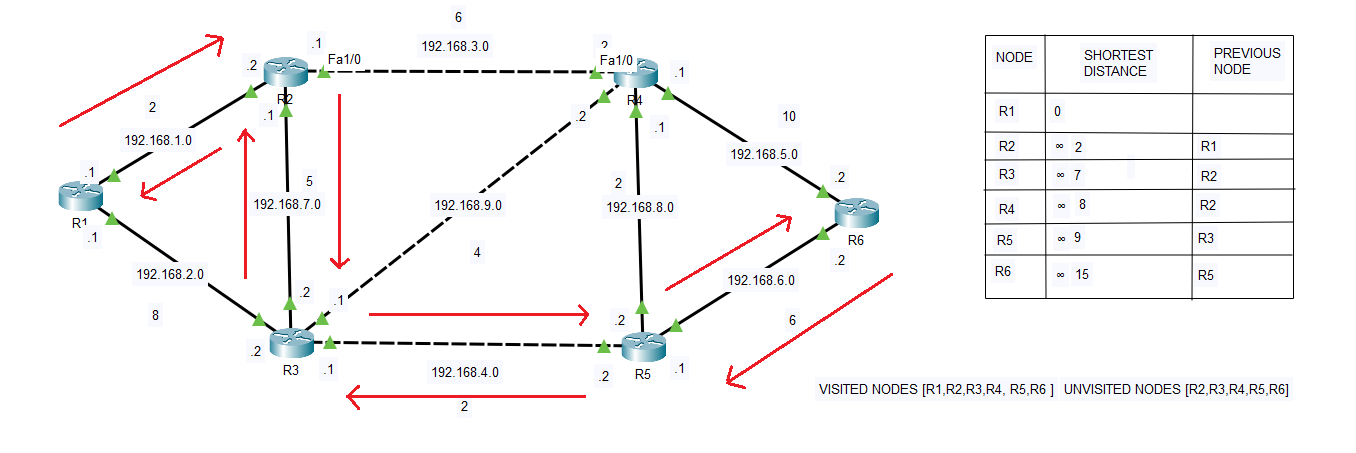
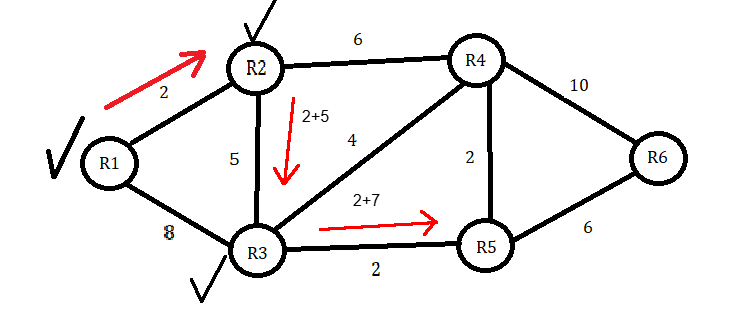
Let’s examine the algorithm and its working process. In the above image, I have configured six routers with OSPF. I have also artificially configured the cost of each interface using the ‘ip ospf cost’ command, followed by the actual cost of the interface. For instance, on interface F0/1 on both R6 and R4, I configured the cost to 5, resulting in a total edge value of 10. For F0/0 interfaces on R5 and R4, the values are set to 1, resulting in a total cost of 2. On each weighted edge, the cost represents an ideal path. The lower the cost, the more desirable the path.
To the right of the lab, I have created a table of tentative values. This table is broken up into three sections: Node, Shortest Distance, and Previous Node. I started with R1, and since it is our starting point, we have all nodes except R1 marked as unvisited; therefore, the starting distance to all other nodes is infinity or unknown, except for R1, which is 0. Initially, the visited nodes section is empty, but it will become full once we find all our paths.
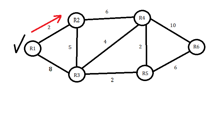
Suppose we start at R1. Between R1 and R2, you can see a cost of 2. From here, we can tell that the price is lower compared to the value of 8 between R1 and R3. In the algorithm, you always want to start your path by choosing the route with the lowest cost to the adjacent node. In this case, it will be the cost between R1 and R2 of 2. We will also compare 2 with the current shortest distance for R2. Since 2 is less than infinity, we will typically replace the infinity symbol with 2. I left the infinity symbols in each box to show the change.
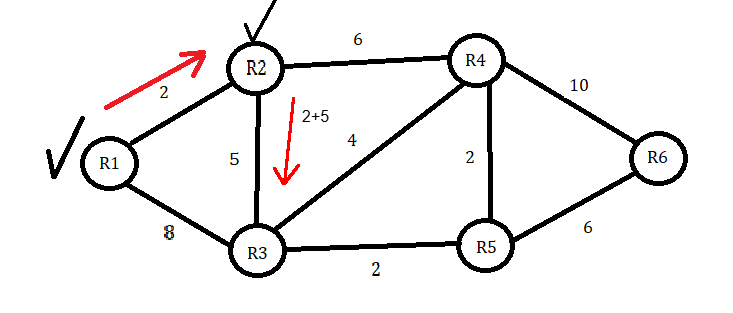
We will now choose the shortest path to the next node, adding the previous value of 2. R2 to R4 is six, so adding 2 would make the total cost 8. If we go to R3 instead, the distance is 5, so 2 plus 5 equals 7. We then conclude that the path to R3 is shorter, so we proceed to the table that corresponds to the shortest distance for R3. Since the distance of 7 is lower than infinity, we will put 7 in the table and R2 as the ‘Previous Node’.
Next, we will put R2 in the ‘Visited Nodes’ box and check it from the ‘Unvisited Nodes’ box. At R3, we now have two choices for unvisited nodes. R4 and R5 are the only path choices available from R3. We now have a total value of 7 at R3 and will add that to the R4 and R5 values. To get to R4, we will add 4 to 7 to get 11. To get to R5, we will add 2 to 7 to get 9. Since 9 is the lower value, we will choose R5 as our next node and mark R3 as visited. Since 9 is less than infinity, it will go under the shortest distance next to R5. R3 will then go into the previous node box.
We only have one Node left, but to ensure that we visit all nodes, we will consider the distance from R4 to R6. In this instance, it’s fairly evident that the distance from R5 straight to R6 is a shorter distance when we add our total of 9 and then 6 to make 15. This is shorter than R5 to R4, which is 2 plus 9, and then adding 10, going from R4 to R6 to make 21.
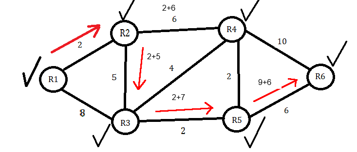
Since 15 is less than infinity, we will write it in the shortest distance next to R6 and mark R5 as visited. We still haven’t visited R4, so we will start back at R2 and go from there to R4. From this, we obtain 8. If we proceed from R4 to R6 and add 10, we arrive at 18. Although 18 is less than infinity, it is still higher than the current shortest distance of 15. Therefore, we will exclude it from the table, but we will mark R4 as visited.
Once the table is completed and all nodes have been visited, it’s just a matter of backtracking our results. Under ‘Node’ on the table, we can start with R6 and proceed to the previous Node, R5. R5 then proceeds to the last R3 node, R3 goes to R2, and subsequently, R2 goes to R1.
This can be done with any visited node, regardless of where we start and end. The entire process has been outlined in this algorithm. For instance, if we begin at R4 and want to know the shortest distance to R1, we only need to use the table. Start at R4, look at the previous Node on the table, which is R2. Then, move from Node R2 to the last Node, R1, for a distance of 8.
Wrapping Up
That’s all for this lab. The algorithm can seem complicated, but it’s pretty simple once you get the hang of it. You can view the path of the OSPF traffic by pinging from each device in simulation mode. You will notice that, every once in a while, the traffic may take an alternate path to load balance. This phenomenon may be something built into OSPF that occasionally bypasses Dijkstra’s Algorithm to add additional efficiency. As always, I have included a link to the Packet Tracer lab on my GitHub repository.
Dijkstra-s-Algorithm/ at main · georgebatton/Dijkstra-s-Algorithm